I collected the audio data from IMEOCAP dataset for the project. It can be downloaded from https://sail.usc.edu/iemocap/.
This dataset contains IEMOCAP emotion speech database metadata in dataframe, and the path to each .wav file.
The Interactive Emotional Dyadic Motion Capture (IEMOCAP) database is an acted, multimodal and multispeaker database,
recently collected at SAIL lab at USC. It contains approximately 12 hours of audiovisual data, including video, speech,
motion capture of face, text transcriptions. It consists of dyadic sessions where actors perform improvisations or scripted
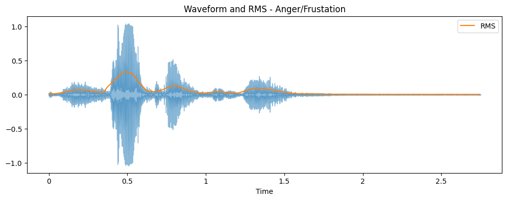
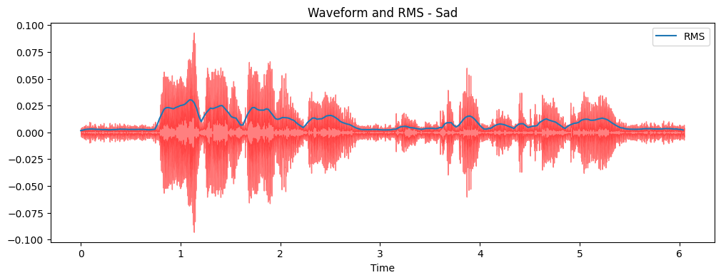
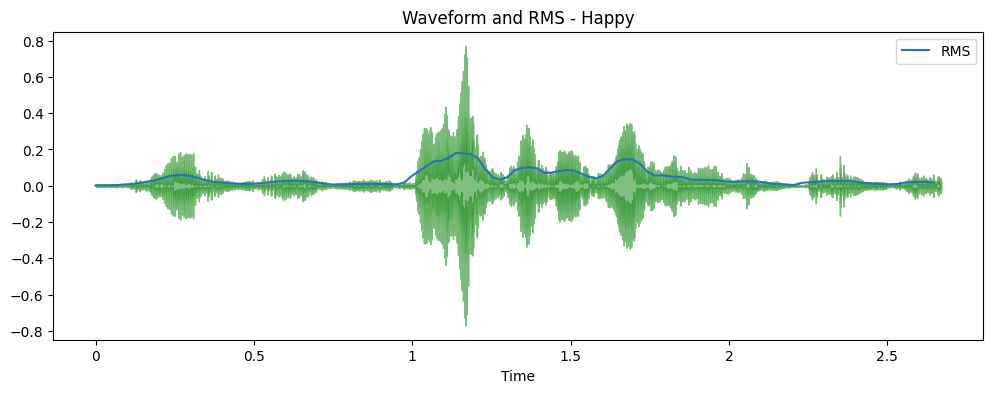
scenarios, specifically selected to elicit emotional expressions. IEMOCAP database is annotated by multiple annotators
into categorical labels, such as anger, happiness, sadness, neutrality, as well as dimensional labels such as valence,
activation and dominance.
To perform analysis and build models I have considered only one session conversation.
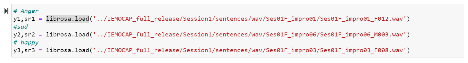
Following is the snapshot what the data looks like.
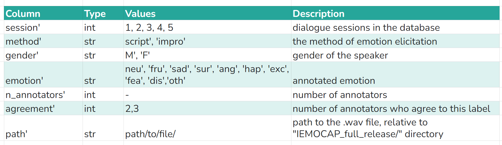
Now in the dataset given, the wav files are in 2 formats.
By nature, a sound wave is a continuous signal, meaning it contains an infinite number of signal values in a given time.
This poses problems for digital devices which expect finite arrays. To be processed, stored, and transmitted by digital devices,
the continuous sound wave needs to be converted into a series of discrete values, known as a digital representation.
The sampling rate (also called sampling frequency) is the number of samples taken in one second and is measured in hertz (Hz).
To give you a point of reference, CD-quality audio has a sampling rate of 44,100 Hz, meaning samples are taken 44,100
times per second.
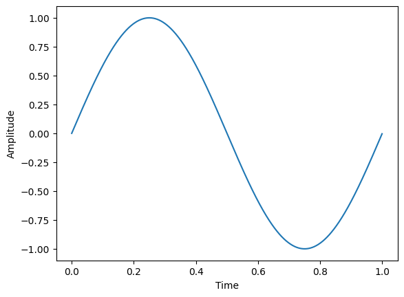
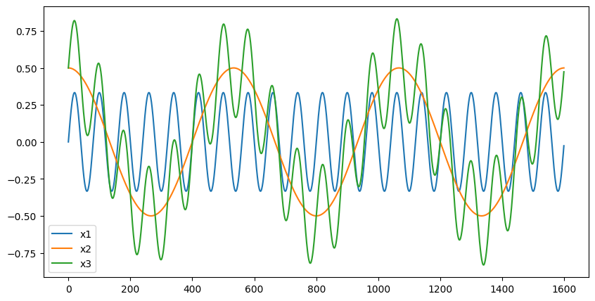
Below shows how a simple sine wave is a continuouswave, a complex wave is mix of sine waves of different amplitude,
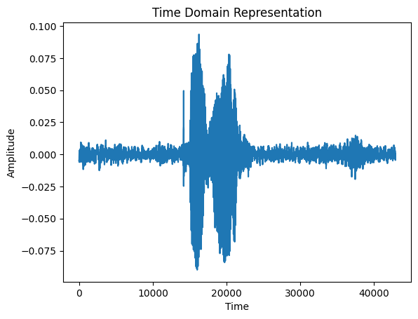
and audio speech wave looks like
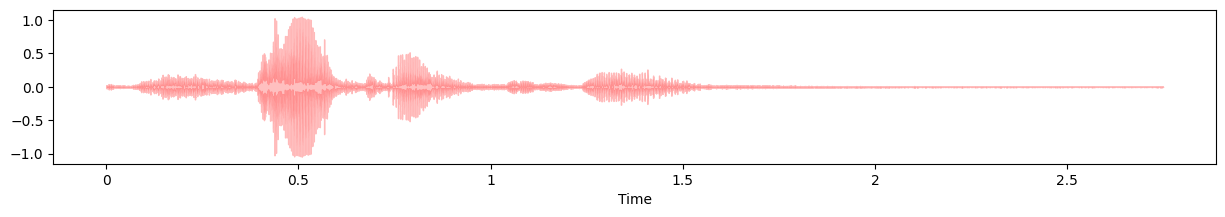
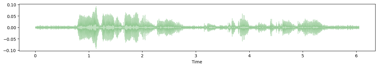
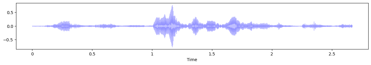
Time Domain representations helps in identifying specific fetures like timing of individual sound events,
the overall loudness of the signal, and any irregularities or noise present in the audio.
The plot shows the amplitude of the signal on the y-axis and time along the x-axis, where each point
corresponds to a single sample value that was taken when this sound was sampled.
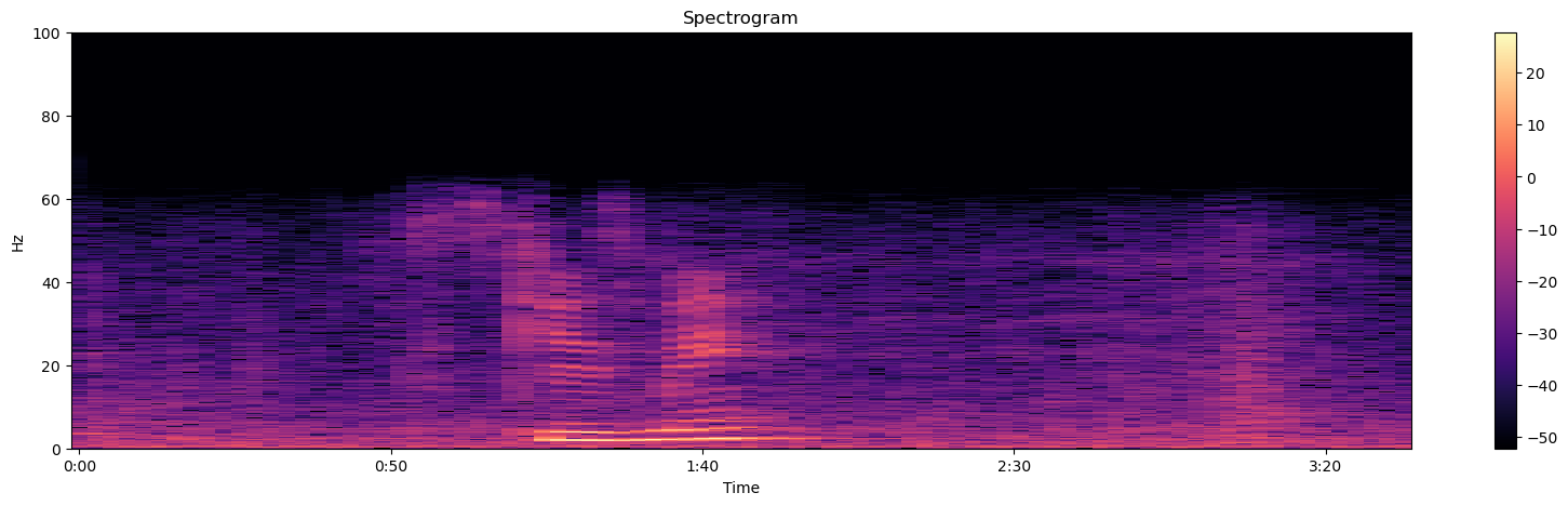
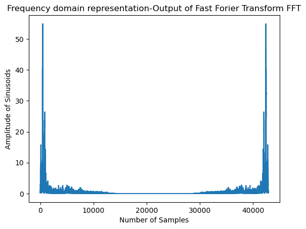
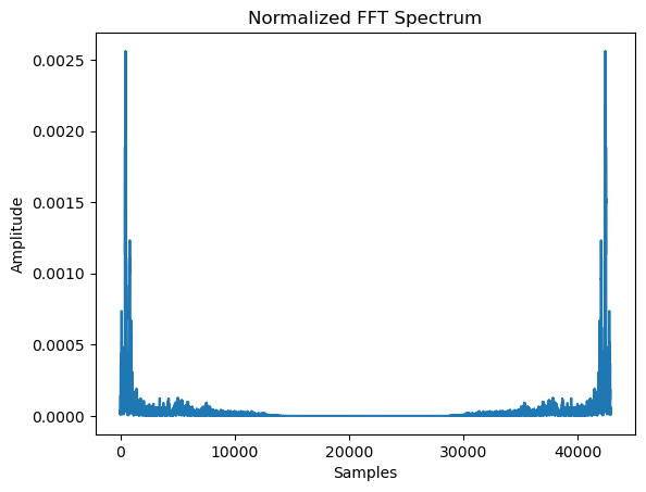
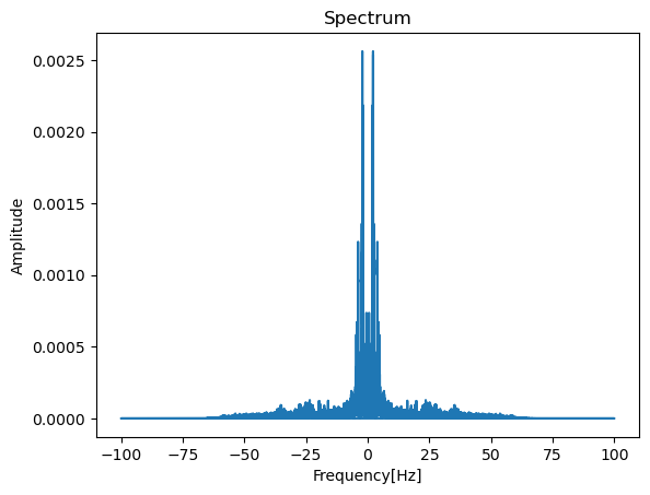
Frequency Domain representations Another way to visualize audio data is to plot the frequency spectrum of an audio signal,
also known as the frequency domain representation. The spectrum is computed using the discrete Fourier transform or DFT.
It describes the individual frequencies that make up the signal and how strong they are.
Learn More on FTT
A microphone records small variations in air pressure (represented by changes in voltage) over time. The ear percieves these slight variations in air pressure as sound. The spectrogram tells us how much different frequencies are present (loudness) in an audio clip at a moment in time.